Such a renown Kaggle competition. Everyone into Machine Learning had tried to predict, who is more likely to survive: be it a family man, a gentlemen with expensive ticket, or a child? Or maybe someone holding a Royalty title? Yes, there is quite a number of features to learn for a machine!
Let’s dive into this tutorial which is more of presentation of my top notch framework for Machine Learning so far! Yes! The framework I’ve build with the courtesy of dataquest.io, spending quite some time getting my best competition results.
Btw, dataquest.io is a great platform and a community to learn some great things!

A typical ML workflow is defined in those steps:
- Data exploration, to find patterns in the data
- Feature engineering and preprocessing, to create new features from those patterns or through pure experimentation
- Feature selection, to select the best subset of our current set of features
- Model selection/tuning, training a number of models with different hyperparameters to find the best performer.
At the end of any cycle we can always submit the predictions for holdout dataset to see the results.
Data Exploration
Data is available on Kaggle Titanic competition page.
A rule of thumb is get acquinted with the domain. Well, reading a wikipage about Titanic is not only fascinating, but can also be beneficial for the competition directly, such as give insight that, for example infants were more likely to survive.
Imports and dataset explorations
import pandas as pd
import numpy as np
import matplotlib.pyplot as plt
%matplotlib inline
train = pd.read_csv('data/train.csv')
holdout = pd.read_csv('data/test.csv')
train.head()
The dataset looks simple enough upon inspecting, and does not have much columns. Kaggle competition page explains all relevant columns.
Let's see survival rate by Sex
```python
sex_pivot = train.pivot_table(index="Sex",values="Survived")
sex_pivot.plot.bar()
plt.show();
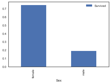
A very vivid barplot.
Survival rate by the ticket classes: 1, 2, 3, where 1-st class is the most expensive.
pclass_pivot = train.pivot_table(index="Pclass",values="Survived")
pclass_pivot.plot.bar()
plt.show();
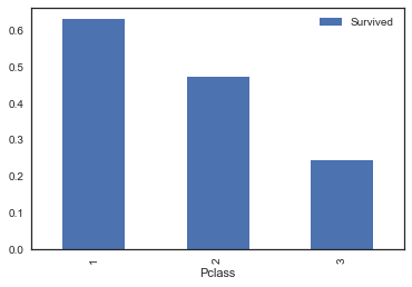
A class disparity is very well seen.
What about age groups?
train["Age"].describe()
count    714.000000
mean      29.699118
std       14.526497
min        0.420000
25%       20.125000
50%       28.000000
75%       38.000000
max       80.000000
Name: Age, dtype: float64
survived = train[train["Survived"] == 1]
survived["Age"].plot.hist(alpha=0.5,color='red',bins=50)
plt.show();
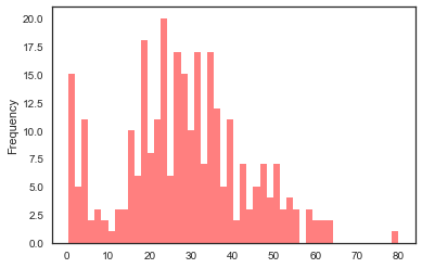
We can see that infants were the first to be saved. Which is obvious if to think about, small babies take least space and people tend to take all of them onboard. Other groups are not that obvious, even though 20-40 years are displayed more frequent than 10 y/olds on the graph, maybe it is just that there were almost no 10 y/olds on Titanic at all?
We should address these questions. A good feature engineering is the next step we are to perform.
Feature engineering
This step is conceived one of the most crucial one. this step is what can reward a scientist with cutting edge prediction percentage. This is where some good thinking is applied.
Clean datasets
A very first, easy step but important step to decide on how to fill those null cells, and ensure overall that all data is consistent.
Turns out there are some missing values in Fare and Embarked columns. Define a function.
def process_missing(df):
    """Handle various missing values from the data set

    Usage
    ------

    holdout = process_missing(holdout)
    """
    df["Fare"] = df["Fare"].fillna(train["Fare"].mean())
    df["Embarked"] = df["Embarked"].fillna("S")
    return df
Create new features
A powerful technique in feature engineering is data binning.
A great example is binning age groups - i.e. assigning each person to a certain group based on their age. pd.cut() is a tool to use for that task.
def process_age(df):
    """Process the Age column into pre-defined 'bins'

    Usage
    ------

    train = process_age(train)
    """
    df["Age"] = df["Age"].fillna(-0.5)
    cut_points = [-1,0,5,12,18,35,60,100]
    label_names = ["Missing","Infant","Child","Teenager","Young Adult","Adult","Senior"]
    df["Age_categories"] = pd.cut(df["Age"],cut_points,labels=label_names)
    return df
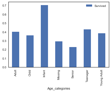
On that step we can draw some deeper insights on survival percentage for age grouped above. We can use again a powerful function df.pivot_table(index='colname1', values='colname2') which would calculate survival means for each age group, giving us surival percentage vividly. Even more we can visualize it.
# Binning by age group
train_copy_df = process_age(train)

# Visualize
age_pivot = train_copy_df.pivot_table(index='Age_categories', values='Survived')
age_pivot.plot.bar()
plt.show();
We can also bin Fare costs to groups.
def process_fare(df):
    """Process the Fare column into pre-defined 'bins'

    Usage
    ------

    train = process_fare(train)
    """
    cut_points = [-1,12,50,100,1000]
    label_names = ["0-12","12-50","50-100","100+"]
    df["Fare_categories"] = pd.cut(df["Fare"],cut_points,labels=label_names)
    return df
Cabins. Looking at cabins we can see each starts with specific letter - might be important. Let’s create features with certain cabin types (start letter). NaN we would replace with ‘Unknown’. Creating a function.
def process_cabin(df):
    """Process the Cabin column into pre-defined 'bins'

    Usage
    ------

    train process_cabin(train)
    """
    df["Cabin_type"] = df["Cabin"].str[0]
    df["Cabin_type"] = df["Cabin_type"].fillna("Unknown")
    df = df.drop('Cabin',axis=1)
    return df
Names contain titles, which can be very important. Let’s extract the titles and assign to certain groups.
def process_titles(df):
    """Extract and categorize the title from the name column

    Usage
    ------

    train = process_titles(train)
    """
    titles = {
        "Mr" :         "Mr",
        "Mme":         "Mrs",
        "Ms":          "Mrs",
        "Mrs" :        "Mrs",
        "Master" :     "Master",
        "Mlle":        "Miss",
        "Miss" :       "Miss",
        "Capt":        "Officer",
        "Col":         "Officer",
        "Major":       "Officer",
        "Dr":          "Officer",
        "Rev":         "Officer",
        "Jonkheer":    "Royalty",
        "Don":         "Royalty",
        "Sir" :        "Royalty",
        "Countess":    "Royalty",
        "Dona":        "Royalty",
        "Lady" :       "Royalty"
    }
    extracted_titles = df["Name"].str.extract(' ([A-Za-z]+)\.',expand=False)
    df["Title"] = extracted_titles.map(titles)
    return df
There is a technique, called create dummies. Above functions serve us to create categories from values. The technique creates a separate feature for each category and got assigned with values 1 or 0 whether a person has this feature or not! This is a very effective technique for Machine Learning.
def create_dummies(df,column_name):
    """Create Dummy Columns (One Hot Encoding) from a single Column

    Usage
    ------

    train = create_dummies(train,"Age")
    """
    dummies = pd.get_dummies(df[column_name],prefix=column_name)
    df = pd.concat([df,dummies],axis=1)
    return df
Now let’s define a function that applies a set of feature-extractions functions to a dataset.
def feature_preprocessing(df):
    df = process_missing(df)
    df = process_age(df)
    df = process_fare(df)
    df = process_cabin(df)
    df = process_titles(df)

    column_name = ['Age_categories', 'Fare_categories', 'Title', 'Cabin_type', 'Sex']
    df = create_dummies(df,column_name)
    return df
Preprocess train and holdout datasets!
train_preprocessed = feature_preprocessing(train)
holdout_preprocessed = feature_preprocessing(holdout)
More Feature Creation
Another cycle of exploration and feature creation.
This time we pay attention to Parch and SibSp columns, which are all about family size of a passenger onboard.
explore_cols = ["SibSp","Parch","Survived"]
explore = train[explore_cols].copy()

explore['familysize'] = explore[["SibSp","Parch"]].sum(axis=1)
pivot = explore.pivot_table(index='familysize',values="Survived")
pivot.plot.bar(ylim=(0,1),yticks=np.arange(0,1,.1));
plt.show();
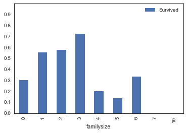
We can see that passengers with higher children count were very likely to survive. While those who had no family aboard had survival chance of only 30%.
Here we create a feature callsed isalone as following:
def isalone(df):
    df['isalone'] = np.where((df['SibSp']==0) & (df['Parch']==0), 1, 0)
    return df
train_preprocessed = isalone(train_preprocessed)
holdout_preprocessed = isalone(holdout_preprocessed)
Great.
We can also create separate features (dummy columns with 1 and 0) for passenger’s Pclass.
train_preprocessed = create_dummies(train_preprocessed,'Pclass')
holdout_preprocessed = create_dummies(holdout_preprocessed,'Pclass')
Drop unnecessary columns
We should get rid of columns we used to derive new features from. Such as Age, Pclass, Fare…
cols_to_drop = ['Age', 'Pclass', 'Fare', 'SibSp', 'Parch']

train_preprocessed = train_preprocessed.drop(cols_to_drop, axis=1)
holdout_preprocessed = holdout_preprocessed.drop(cols_to_drop, axis=1)
Postprocessing
- Ensure no NA columns are in the dataset.
- Also ensuring to select columns only with numerical data - an important processing step for ML.
- Preprocessing - minmax normalization.
from sklearn.preprocessing import minmax_scale

def only_numeric(df):
    df = df.dropna(axis=1)
    df = df.select_dtypes(include=[np.number])

    return df

#minmaxnormalization here if required. If there are columns left with varying values.
#train_rescaled = pd.DataFrame(minmax_scale(train[cols_to_rescale]), columns=cols_rescaled)
train_preprocessed = only_numeric(train_preprocessed)
holdout_preprocessed = only_numeric(holdout_preprocessed)
Feature selection
RFECV - recursive feature selection! It automatically selects best columns for a model of choice.
Example:
from sklearn.feature_selection import RFECV
from sklearn.ensemble import RandomForestClassifier

def select_features(instantiated_model, all_X, all_y):

    clf = RandomForestClassifier(random_state=1)

    selector = RFECV(instantiated_model, cv=10, scoring='roc_auc')
    selector.fit(all_X, all_y)
    optimized_columns = all_X.columns[selector.support_].values
    print(optimized_columns)

    return optimized_columns
Note: in practice RFECV feature selector is not very useful, unfotunately worsens performance so far in my experience.
Diminish collinearity
Collinearity happens when a values in one column can be derived from another. For example male/female columns which obviously complement each other. Person can be either male or female. Collinearity effects can be seen in multiple columns also.
To diminish collinearity we can simply drop one of the columns in a pack.
Which columns have correlinearity? We would first visualize correlation for columns and then select which to drop. Here is a nice function which highlights collinear columns with deeper color:
# Drop certain columns that complement each other
import numpy as np
import seaborn as sns

def plot_correlation_heatmap(df):
    corr = df.corr()

    sns.set(style="white")
    mask = np.zeros_like(corr, dtype=np.bool)
    mask[np.triu_indices_from(mask)] = True

    f, ax = plt.subplots(figsize=(16, 14))
    cmap = sns.diverging_palette(220, 10, as_cmap=True)


    sns.heatmap(corr, mask=mask, cmap=cmap, vmax=.3, center=0,
            square=True, linewidths=.5, cbar_kws={"shrink": .5})
    plt.show()
plot_correlation_heatmap(train_preprocessed)
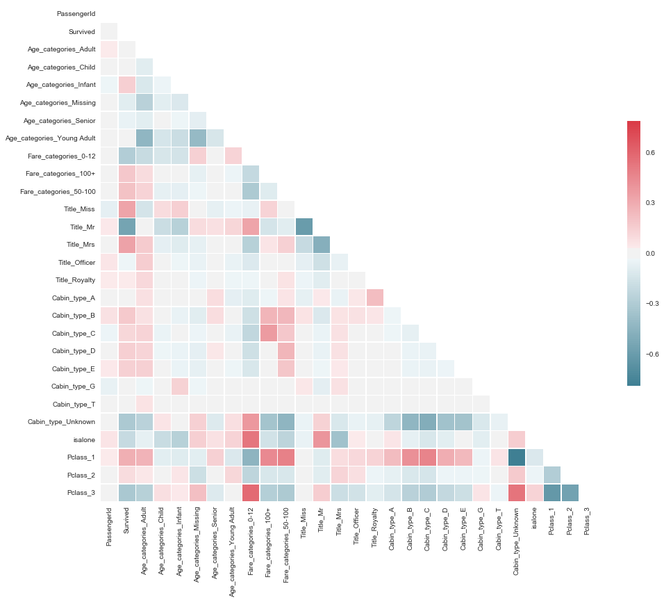
Ok, obviously Sex_female/Sex_male and Title_Miss/Title_Mr/Title_Mrs are very salient on the heatmap. We’ll remove Sex_female/male completely and leave out Title_Mr/Mrs/Miss as more nuanced.
Apart from that, we should remove each of the following from the corresponding groups:
- Cabin_type_F
- Age_categories_Teenager
- Fare_categories_12-50
- Title_Master
cols_to_drop = ['Sex_male','Sex_female','Cabin_type_F','Age_categories_Teenager','Fare_categories_12-50','Title_Master']
train_preprocessed = train_preprocessed.drop(cols_to_drop, axis=1)
holdout_preprocessed = holdout_preprocessed.drop(cols_to_drop, axis=1)
Model Selection and Tuning!
Now this is fun part! This is where we build (train) our models. That is usually quite exciting to choose those great algorithms out there and see it performing great (at least sometimes!). This is where we see Machine Learning in work. Magic!
Split datasets for ML
At this point split dataframes into all_X and all_y (data and labels) properly. That’s what we’ll be feeding into models.
all_X, all_y = train_preprocessed.drop(['Survived','PassengerId'], axis=1), train_preprocessed['Survived']
test_X = holdout_preprocessed
Ensure at this point that featurelist (column names) coincide. As it may happen so, that some categories are absent in holdout dataset. So, we have to use those columns, which both datasets share for sure.
# Grab all available colnames from all_X to use as a column_list
column_list = list(all_X.columns.values)
# Ensure all colnames in the list is present in holdout collist name. Choose only those that coincide.
col_list_to_choose_from = list(test_X.columns.values)
columns = [colname for colname in column_list if colname in col_list_to_choose_from] # Such mumbo jumbo is required because not all columns are the same in the holdout dataset
Now let’s use these columns further on. It helps to avoid possible issues.
all_X = all_X[columns]
GridSearch best hyperparameters and model!
Now we’ll create a function to do the heavy lifting of model selection and tuning. The function will use three different algorithms and use grid search to train all combinations of hyperparameters and find best performing model!
from sklearn.model_selection import GridSearchCV
from sklearn.neighbors import KNeighborsClassifier
from sklearn.linear_model import LogisticRegression
from sklearn.ensemble import GradientBoostingClassifier
A list of parameters!
It can be achieved by creating a list of dictionaries— that is, a list where each element of the list is a dictionary. Each dictionary should contain:
- The name of the particular model
- An estimator object for the model
- A dictionary of hyperparameters that we’ll use for grid search.
Example of list of dictionaries (hyperparameters that gidsearch will use) can look like:
# Define a list of dictionaries, that describe models and their parameters we want gridsearch for the best param!
list_of_dict_models = [
    {
        'name':'LogisticRegression',
        'estimator':LogisticRegression(),
        'hyperparameters':
        {
            "solver": ["newton-cg", "lbfgs", "liblinear"],
            'C':[0.6, 0.7, 0.8, 0.9, 1, 1.2, 1.5],
            'tol':[0.001, 0.01, 0.1, 0.5, 1, 5]

        }
    },

    {
        'name':'KNeighborsClassifier',
        'estimator':KNeighborsClassifier(),
        'hyperparameters':
        {
            "n_neighbors": range(1,20,2),
            "weights": ["distance", "uniform"],
            "algorithm": ["ball_tree", "kd_tree", "brute"],
            "p": [1,2]
        }
    }
]
Now that we have a dictionary of different models. Let’s create a function that would gridsearch through all of them and find best params!
It should return an updated dictionary. And also printing in a nice way it’s findings.
Note: it contains RFECV feature selector, commented though, as it proved not very useful last time.
def select_model(all_X, all_y, list_of_dict_models):
    this_scoring = 'accuracy'
    for model in list_of_dict_models:
        print('Searching best params for {}'.format(model['name']))
        estimator = model['estimator']

#         # First Recursive column selection for each model
#         if model['name'] not in ['KNeighborsClassifier']:
#             selector = RFECV(estimator, cv=10, scoring=this_scoring)
#             selector.fit(all_X, all_y)
#             optimized_columns = all_X.columns[selector.support_].values
#             model['optimized_columns'] = optimized_columns
#             print('col_list lenght: {}'.format(len(optimized_columns)))

        grid = GridSearchCV(estimator, param_grid=model['hyperparameters'], cv=10, scoring=this_scoring, n_jobs=-1)
        grid.fit(all_X, all_y)

        model['best_hyperparameters'] = grid.best_params_
        best_score = grid.best_score_
        model['best_score'] = best_score
        model['best_estimator'] = grid.best_estimator_


    list_of_dict_models_sorted_best = sorted(list_of_dict_models, key=lambda x: x['best_score'], reverse=True)
    best_model = list_of_dict_models_sorted_best[0]['name']
    best_score_achieved = list_of_dict_models_sorted_best[0]['best_score']
    print('Best Model: {}, score: {}'.format(best_model,best_score_achieved))


    return list_of_dict_models_sorted_best
Run the powerful search function! Get the dictionary.
list_of_dict_models_sorted_best = select_model(all_X, all_y, list_of_dict_models)
Searching best params for LogisticRegression
Searching best params for KNeighborsClassifier
Best Model: LogisticRegression, score: 0.813692480359147
Additionally print the whole dictionary (for exploration purposes)
print(list_of_dict_models_sorted_best)
[{'name': 'LogisticRegression', 'estimator': LogisticRegression(C=1.0, class_weight=None, dual=False, fit_intercept=True,
          intercept_scaling=1, max_iter=100, multi_class='ovr', n_jobs=1,
          penalty='l2', random_state=None, solver='liblinear', tol=0.0001,
          verbose=0, warm_start=False), 'hyperparameters': {'solver': ['newton-cg', 'lbfgs', 'liblinear'], 'C': [0.6, 0.7, 0.8, 0.9, 1, 1.2, 1.5], 'tol': [0.001, 0.01, 0.1, 0.5, 1, 5]}, 'best_hyperparameters': {'C': 0.6, 'solver': 'newton-cg', 'tol': 0.001}, 'best_score': 0.81369248035914699, 'best_estimator': LogisticRegression(C=0.6, class_weight=None, dual=False, fit_intercept=True,
          intercept_scaling=1, max_iter=100, multi_class='ovr', n_jobs=1,
          penalty='l2', random_state=None, solver='newton-cg', tol=0.001,
          verbose=0, warm_start=False)}, {'name': 'KNeighborsClassifier', 'estimator': KNeighborsClassifier(algorithm='auto', leaf_size=30, metric='minkowski',
           metric_params=None, n_jobs=1, n_neighbors=5, p=2,
           weights='uniform'), 'hyperparameters': {'n_neighbors': range(1, 20, 2), 'weights': ['distance', 'uniform'], 'algorithm': ['ball_tree', 'kd_tree', 'brute'], 'p': [1, 2]}, 'best_hyperparameters': {'algorithm': 'brute', 'n_neighbors': 3, 'p': 1, 'weights': 'uniform'}, 'best_score': 0.8125701459034792, 'best_estimator': KNeighborsClassifier(algorithm='brute', leaf_size=30, metric='minkowski',
           metric_params=None, n_jobs=1, n_neighbors=3, p=1,
           weights='uniform')}]
Generate output
A function that generates final output for Kaggle submission. As an input it takes a trained model, colnames, and optional filename to save to.
def save_submission_file(best_trained_model, colnames, filename='latest_submission.csv'):

    test_y = best_trained_model.predict(test_X[colnames])
    submission = pd.concat([test_X['PassengerId'],pd.Series(test_y,name='Survived')], axis=1)
    #submission.rename(columns={0:'Survived'}, inplace=True)
    #print(submission.head(3))
    submission.to_csv(filename, index=False)
Retrive best performing model from the dictionaries (or a model of choice).
And thus we are ready to run a function, to get a latest file for a submission!
Dataset looks fine and abundant with columns. Let’s assign proper data to test_X.
# Alternatively just grab all available colnames from all_X to use as a column_list
column_list = list(all_X.columns.values)
#column_list.append('PassengerId')
best_trained_model = list_of_dict_models_sorted_best[0]['best_estimator']
save_submission_file(best_trained_model, column_list, filename='latest_submission.csv')
The output ready for Kaggle submission would be saved locally as filename!
Good Luck!
Hope some techniques as well as the framework is most helpful for your endeavors. Have great Machine Learning experience!